|
|
ParaView (ParaView Website) is an open-source application for visualizing two- and three-dimensional data sets. It is a multi-platform parallel data analysis and visualization application built upon the Visualization Toolkit (VTK) library. It can process very large data sets in parallel and later collect the results using a parallel machine. It helps in visualizing simulation results from simulations run on supercomputing resources that are often too big for a single desktop machine to handle. To enable interactive visualization of such datasets, it uses remote and/or parallel data processing. The basic concept is that if a dataset cannot fit on a desktop machine due to memory or other limitations, we can split the dataset among a cluster of machines, driven from the desktop.
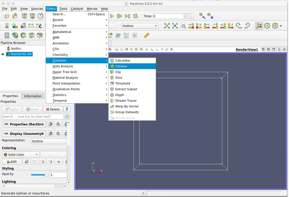
 2. Now, create a contour inside the rectangle. Click on Filters -> Common -> Contour. Now a countour1 will be created under the Pipeline Browser section.
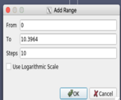
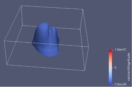
 3. After the contour1 is created, now go to Properties -> Isosurfaces. Remove the value in the “Values Range:” using the – (minus sign) adjacent to the section. Now, click on the scale-like button just below the – (minus sign). Click “ok” in the dialog box. Refer to below screenshot:
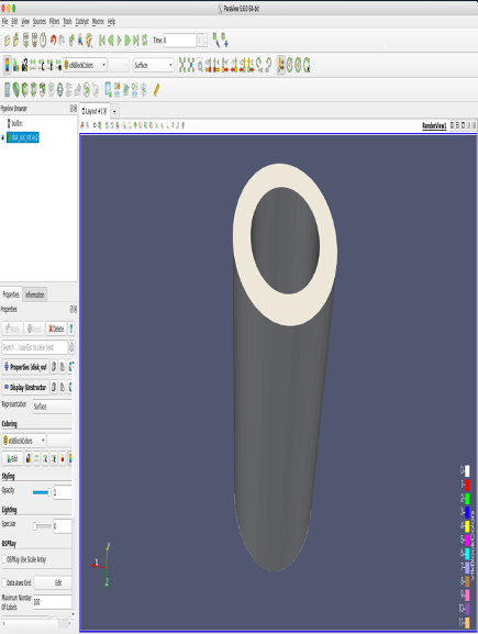
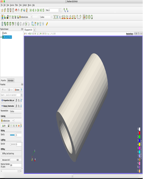
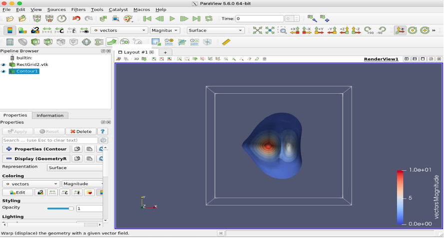
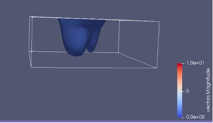
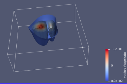
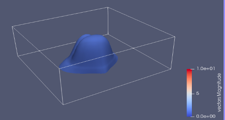
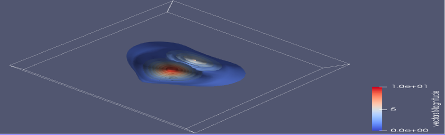
 4. Go to Contour1 -> Properties -> Coloring -> vectors (from solid color). Use mouse to rotate the output and visualize the 3-D object.
Steps to Run ParaView GUI From The Terminal
1. Login to the Arc system on the terminal using the sample command shown below: $ ssh -X username@arc.utsa.edu$ srun --x11 -p compute1 -t 8:00:00 -n 1 -N 1 --pty bash$ ml paraview
$ paraview --mesa
Cylinder Visualization Example
1. Copy the data files to your working directory from the ParaView example directory: $ cp -r /apps/paraview/examples/ .Contour In Rectangle Visualization Example
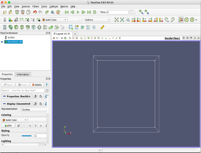
1. Open the file rect_grid2.vtk from the data directory, and click Apply.- This file will display a rectangle shown below:
2. Now, create a contour inside the rectangle. Click on Filters -> Common -> Contour. Now a countour1 will be created under the Pipeline Browser section.
3. After the contour1 is created, now go to Properties -> Isosurfaces. Remove the value in the “Values Range:” using the – (minus sign) adjacent to the section. Now, click on the scale-like button just below the – (minus sign). Click “ok” in the dialog box. Refer to below screenshot:
4. Go to Contour1 -> Properties -> Coloring -> vectors (from solid color). Use mouse to rotate the output and visualize the 3-D object.
References
Edit | Attach | Print version | History: r4 < r3 < r2 < r1 | Backlinks | View wiki text | Edit wiki text | More topic actions
Topic revision: r4 - 24 Sep 2021, AdminUser
- Toolbox
-
 Create New Topic
-
 Index
Index
-
 Search
-
 Changes
-
 Notifications
-
 RSS Feed
-
 Statistics
-
 Preferences
Ideas, requests, problems regarding Foswiki? Send feedback